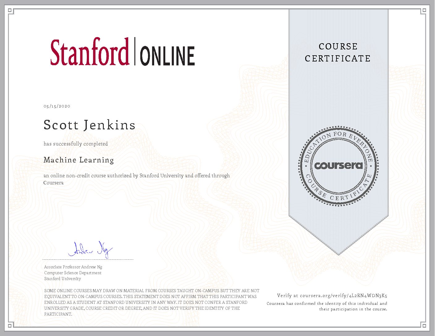
In this post, I write in reflection of the Machine Learning course I finished this week, and demonstrate how I was able to use some of this content to build a more accurate regression model for predicting house prices.

Machine Learning Course 

Andrew Ng’s Coursera Machine Learning course is widely acclaimed by the data science community. On the positivity of reviews alone, I decided to devote some lockdown time to its study. The 56 hour course is chunked into 11 topics, which I tackled at roughly 2 a week. The course covers both supervised and unsupervised learning, as well as recommended practices for machine learning implementation. It was assessed through programming assignments in GNU Octave and online quizzes.

Topics covered include:

• Linear Regression 
• Logistic Regression
• Regularisation
• Neural Networks
• Bias/Variance Theory
• Support Vector Machines
• Dimensionality Reduction
• Collaborative Filtering Recommendation System

Taking notes throughout the course felt a lot like returning to university, only with the delight of not having to sit an exam at the end! Having recently skim read my old Matlab notes, I didn’t have much trouble with the Octave programming exercises and found them fairly hand-holding. Whilst this is perhaps best for an online course with no face to face support, I was keen to concurrently apply some of the content in Python.

Kaggle House Prices

Since Regression was the first topic in the course, I decided to pick out a regression competition on Kaggle. This House Price Prediction problem (LINK) looked perfect. Dozens of features would allow me to practice cleaning, feature engineering, and particularly, my new knowledge of the Bias-Variance tradeoff and parameter regularisation. I have uploaded my Jupyter notebook to GitHub.

I find breaking data cleaning down into separate pre-processing steps keeps me focused on what otherwise can be a soul-crushing task! Additionally, taking on the mindset of a detective adds interest to this stage. Why is that an outlier? Why could those values be missing? Does this correlation make sense? Numerous ‘Aha!’ moments offer punctuation of this chapter. My approach was as follows:

1. Check for and remove any outliers from the training set.
2. Check for skew and transform target variable (House Price) to have Normal Distribution.
3. Concatenate Train and Test sets to create a single frame to clean. Note that this is the easiest and quickest way to ensure that my train and test sets have the same features after cleaning.
4. Handle missing values through dropping columns or data imputation as appropriate.
5. Check for correlation between independent variables and remove any with high (> 0.9) collinearity.
6. Consider binning categorical variables to create more helpful features.
7. Apply one-hot encoding on categorical variables.
8. Split clean frame back into train and test splits.

It is good practice to scale numerical features to obey a Gaussian (0,1). This is often performed as part of model building.

I was particularly pleased with the following 2 heatmap visualisations in this section. First, showing which columns contained null values.

Second, using the mask parameter to produce a triangular output with very clear colouring.

Moving onto the modelling, I was impressed with the improvement regularisation made to the RMSE of the predictions – 0.12 with hyperparameter tuning down from 0.28 without regularisation.

I was pleased to apply some of the Variance/Bias theory to select an appropriate penalty alpha for the regularised regression. High variance models overfit the training set, resulting in low RMSE on the training examples but high RMSE on new examples the model wasn’t trained on. We see that this is the case on models with low alpha. This makes sense: With no penalty on parameter size, the model will produce a better fit on the training data.

Our aim is to build a model which performs well on new examples in the test set. That is, choose alpha where the validation error (red line) is small. Hyperparameter tuning moved my model up 500 places on the leaderboard (a 0.5 improvement on RMSE.)

What Next?

From this course, I have 3 outputs.

I value being able to practice what I learn, and find a tangible output motivating. As such, I’m keen to apply other content in this course (Logistic Regression, Dimensionality Reduction, SVM’s) to a classification problem.

I’ve written previously about product sequencing. The collaborative filtering method introduced in this course is a method which could be used in this domain which I am interested to learn more about.

Finally, I applied my first neural networks in Octave in this course, and am keen to get started with TensorFlow in Python to take this further.

There is certainly no shortage of material to explore whilst I’m on the bench. 

Until Next Time,

Scott