In this post, I write about methods to answer 3 important questions in the field of store space optimisation. I aim to identify the constraints of each model, and comment on other considerations which should come into play when devising a store layout.

Brief

Retail stores can serve multiple purposes. Primarily, they drive sales for the business as transactional spaces. Additionally, they can serve as destinations of inspiration – browsing customers are able to experience the range before purchasing online. Thirdly, they serve as adverts to increase brand awareness among people who are not current customers. 

In my writing today, I focus on a store’s purpose as a transactional space, and how space analytics can make refit suggestions aimed at maximising sales through adjusting the floorplan alone.. 

One way to increase sales could be to increase the size of the store. A larger store can hold a wider range of products or a deeper inventory; better availability for the customer. But a larger store will also cost more in rent, which is usually charged at a fixed rate by the square foot.. And whilst a larger store may generate more sales, we will quickly meet a level of diminishing returns. Making the average store 10% larger may generate around 10% more sales, but a store 50 times the size will not return sales anywhere near 50 times its current levels.

The metric I use in this post is the Trading Intensity (TI) which is calculated as:

Increasing the TI is a challenge of working the space harder; increasing the sales from a space of fixed size. From a modelling perspective, it is helpful to think of a store as a box with constant dimensions. We can choose which products to put into the box and in what ratio. We make ongoing observations of what customers are buying and can adjust the box contents in response or anticipation to this. We have flexibility in the size and position of the contents as well. 

Department Adjacencies: Which departments should be next to each other?

Why would it matter which departments are next to each other? It is an opportunity for retailers to make it easier for their customers to shop the store and keep customers happy. Imagine a store where all of the products are lined up randomly on the shelves. Would you shop there? I wouldn’t – think how difficult it would be to find anything! It is also an opportunity for cross-selling.

I outline a data-led method of how retailers can do better than the random catastrophe described above.

Begin by running market basket analysis at a department level for each store. Basket analysis allows us to determine which products are most frequently bought together; for a clear explanation of the apriori algorithm try this page. For each store, tabulate the lift for each pair of departments, by either volume or value. 

Next, define a proximity function for two departments, a measure of how ‘close’ together these departments are. This could be done in a number of ways, considerations may include midpoints, shared edges, walking distance, euclidean distance, aisle widths. Any sensible logic works as a good first pass. For added mathematical consistency, we could consider the set of departments to be a metric space and define the proximity function to meet the criteria of a metric. A further development could be more customer-centric. Tracking how customers flow through a store with heat mapping would be another lens through which to view department adjacencies.

A clear visual is often useful in graph theory, and in Python, the Networkx package is the tool for the job. Given a store plan and the definition of adjacency, we can produce a department adjacency graph, such as the one mocked up below. Applying Djikstra’s algorithm will output the shortest path for each pair of departments.

In the above example with a uniform edge weight of 1, we have

Proximity (Utility, Storage) = 2

Proximity (Dining, Bathroom) = 5

With this data collected for all stores, plot the lift against proximity for each pair of departments. In the graphs below, each cross represents a different store. We expect to find that as departments are moved further from each other, they are less likely to be found in the same basket, and so the lift decreases.

Now, here’s the decision making power. Different pairs of departments will have lift values with different sensitivities to proximity. That is to say that the lift value of one pair of departments may drop off much faster than the lift value of another pair.

When planning a store layout, it makes sense to prioritise the adjacency of departments with the most sensitive lift values. Case closed? Not quite. This can be extended further through factoring in the departmental average item value in mixed baskets.

Plotting the derivative of lift with respect to proximity (how quickly the curve drops off) with department value will produce the following matrix. In the below graph, each cross represents a pair of departments. Note that we consider -d/dp (Lift) in this graph.

Ensure pairs of departments of high value which have a lift heavily impacted by proximity are the first to be positioned next to each other. Low value departments which have their lift impacted least by the proximity to other departments are the ones to position last; their performance is not adversely affected by neighbouring departments.

With an idea on which departments to have neighbouring each other, let’s now consider how to position departments within a store.

Where to put departments?

Ever wondered why the milk and bread is furthest from the door in a supermarket. It’s not an accident. Supermarkets put their best selling products at the back in the hope that you’ll add multiple things to your basket along the way. Similarly, you’ll find a stand of batteries and gift cards near the tills; these products are more likely to be bought here, than anywhere else in the store.

We can extend the adjacency method above to give insight on department positioning as well, by defining the door as a separate department. But since the door doesn’t generate any sales (it’s just a door!), lift is not an appropriate metric. 

For each store and each department calculate the Trading Intensity. Better results may arise from normalising sales or footfall across stores to prevent trends being dominated by larger stores across an estate.  Use a proximity function to calculate the distance between the department and the entrance. As an example across 2 stores and 3 departments:

Store	Department	TI	Proximity
X	A	5	1
X	B	3	2
X	C	2	3
Y	A	2	2
Y	B	2.5	3
Y	C	2	1

For each Department, plot the curve of Trading Intensity against Proximity.

For departments with a TI highly impacted by proximity to the door, it makes sense to put these near the entrance, in the above example, Department A. Departments with little relation between TI and Proximity can be added last, safe in the evidence that their location will not make much difference to their sales, in the above example, Department C. It may also be relevant to apply this method to assess a department’s distance from the tills, from an in-store cafe, or from the warehouse (factoring in the replenishment rate and corresponding value of the store colleagues time.) 

With our departments in place and their neighbours established, let’s move on to the allocation of floor space.

Department Sizing: How much space to allocate to each department

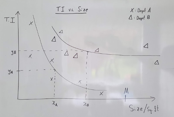
Take our Trading Intensity values calculated at department level for each store and plot them against department size. In the below example in the 2 department case, I have drawn curves for interpretability, though regression lines could be found with an appropriate transform. In the graph below, each cross represents Department A for a different store, and each triangle represents Department B for a different store. 

With sales normalised for footfall, we expect to see an inversely proportional relationship between TI and Size. The extrapolated curves of best fit will be different for each department depending on product dimensions and sell-through rate.

 We want to solve the following algebraic optimisation problem under certain constraints:

This is the case with only two departments, but it easily generalises. We want to maximise the store sales. One limitation is that all the departments must fit within the store! We may also choose to impose conditions on the minimum and maximum sizes of each department to ensure that we have a reasonable selection for customers. Presented as above, this is a linear programming problem. The simplex algorithm is usually sufficient to solve small problems.

Above, we have modelled space on a continuous scale, and a valid output could be to assign 765.61 square feet to department A and 234.39 square feet to department B. Is this helpful? Not really.

A practical difficulty with this method is product ranging. For consistency across stores and easier merchandising, we may choose to restrict the possible sizes of each department to a handful of prescribed values. Solving the revised problem with discrete allowable sizes for each department is now a variation of the Knapsack problem. It’s NP-Complete (Boo! There is no known polynomial time algorithm solution.) Dominant relations can only prune our department set so far. So while this may model the store better, it is far more computationally expensive.

Other Considerations:

• Online Halo. Store sales alone may not be the correct metric.
• Assembling the finished jigsaw! Any solutions found through the above method serve as guidelines only and will need to be adjusted. We haven’t considered department shape, walkway and aisle widths. While interesting, I expect that we will quickly reach a point of diminishing returns.

If you’ve read this far, I hope you have a clearer understanding of the preceding logic for store space planning. Ironically, I’m writing this at a time when most non-retail stores are closed and such experiments can not take place. Further, I wonder whether the forced shift to ecommerce during lockdown will prove to be a catalyst in changing customer behaviour. An understanding of the store-web relationship and the online halo could be even more pertinent in the future..

Until Next Time,

Scott